Hermite-Simpson Collocation for Solving ODEs
Hermite-Simpson collocation is a numerical method to solve continuous-time Ordinary Differential Equations (ODEs) using piecewise cubic Hermite polynomials and Simpson quadrature. Simpson quadrature approximates the integrand using a quadratic interpolating polynomial and integrates this polynomial exactly. When both these methods are combined to discretize the differential equation, it leads to well-known Hermite-Simpson collocation. Though widely used in context of trajectory optimization, for brevity the discussion here is limited to solving stiff initial-value problems. The Hermite-Simpson collocation is also an implicit Runge Kutta integrator.
Initial value problem
An initial value problem (IVP) consists of a differential equation $\dot{x} = f(t, x)$ defined over $t \in [t_0, t_f]$ and an initial condition $x(t_0) = x_0$. Assuming $f$ is sufficiently regular to guarantee existence and uniqueness, the IVP can be written in its integral form as $x(t)=x(t_0)+\int_{t_0}^{t}f(\tau,x(\tau)) d \tau$
Derivation of the collocation equations
Divide the intervals $t \in [t_0,t_f]$ into $N$ uniform sub-intervals of width $h=\frac{t_f-t_0}{N}$. Let $t_i$, $x_i$ and $f_i$ denote the discrete value of the time, state and state derivative at point $i \in {1,\dots,N+1}$. On the i-th sub-interval, integrating the ODE and approximating the right-hand side using Simpson quadrature yields,
$\int_{t_i}^{t_{i+1}}\dot{x}dt=\int_{t_i}^{t_{i+1}}f~\mathrm{d} \tau$
$x_{i+1}-x_i=\int_{t_i}^{t_{i+1}}f~\mathrm{d} \tau$
$\int_{t_i}^{t_{i+1}}fdt=\dfrac{h}{6}\left(f_i+4f_{i+\frac{1}{2}}+f_{i+1}\right)$
where $i+\frac{1}{2}$ denotes the value at the midpoint of the i-th interval. To determine $f_{i+\frac{1}{2}}$, the value of the state at this point must be determined. The state on each sub-interval is approximated by a cubic Hermite polynomial, which is uniquely determined by the state and derivative values at the two endpoints. The derivation of the coefficients of the cubic Hermite interpolation polynomial is shown below.
Hermite interpolant
$x(\tau) \approx a\tau^3+b\tau^2+c\tau+d$
$x(0)=a0^3+b0^2+c0+d$
$x(h)=ah^3+bh^2+ch+d$
$\dot{x}(0)=3a0^2+2b0+c$
$\dot{x}(h)=3ah^2+2bh+c$
The boundary conditions at node $i$ determine the coefficients $c$ and $d$. Substitute the values in the remaining equations and solve for $a$ and $b$. The matrix form is retained to simplify the derivation in the later section.
\[\begin{bmatrix} h^3 &h^2\\ 3h^2 &2h \end{bmatrix} \begin{bmatrix} a\\ b \end{bmatrix} =\begin{bmatrix} x(h)-\dot{x}(0)h-x(0)\\ \dot{x}(h)-\dot{x}(0) \end{bmatrix}= \begin{bmatrix} x_{i+1}-f_ih-x_i\\ f_{i+1}-f_{i} \end{bmatrix}\] \[\begin{bmatrix} a\\ b \end{bmatrix}=\dfrac{-1}{h^4} \begin{bmatrix} 2h &-h^2\\ -3h^2 &h^3 \end{bmatrix} \begin{bmatrix} x_{i+1}-f_ih-x_i\\ f_{i+1}-f_{i} \end{bmatrix}\]To compute $x_{i+\frac{1}{2}}$, evaluate the cubic Hermite polynomial at the midpoint of the interval. Upon simplification, this leads to an expression for the state at the midpoint in terms of the values at the boundaries of the sub-interval. \(\begin{aligned} x(\frac{h}{2}) &=x_{i+\frac{1}{2}}\\ &=a\dfrac{h^3}{8}+b\dfrac{h^2}{4}+c\dfrac{h}{2}+d\\ &= \begin{bmatrix} \dfrac{h^3}{8}&\dfrac{h^2}{4} \end{bmatrix} \begin{bmatrix} a\\ b \end{bmatrix} + f_i\dfrac{h}{2}+x_i\\ &= \begin{bmatrix} \dfrac{h^3}{8}&\dfrac{h^2}{4} \end{bmatrix} \dfrac{-1}{h^4} \begin{bmatrix} 2h &-h^2\\ -3h^2 &h^3 \end{bmatrix} \begin{bmatrix} x_{i+1}-f_ih-x_i\\ f_{i+1}-f_{i} \end{bmatrix} + f_i\dfrac{h}{2}+x_i\\ &= \dfrac{-h^4}{h^4} \begin{bmatrix} (\dfrac{1}{4}-\dfrac{3}{4})&(\dfrac{-1}{8}+\dfrac{1}{4}) \end{bmatrix} \begin{bmatrix} x_{i+1}-f_ih-x_i\\ f_{i+1}-f_{i} \end{bmatrix} + f_i\dfrac{h}{2}+x_i\\ &= \begin{bmatrix} \dfrac{1}{2}&\dfrac{-h}{8} \end{bmatrix} \begin{bmatrix} x_{i+1}-f_ih-x_i\\ f_{i+1}-f_{i} \end{bmatrix} + f_i\dfrac{h}{2}+x_i\\ &= \dfrac{x_{i+1}}{2}-\dfrac{f_ih}{2}-\dfrac{x_i}{2}+ \dfrac{f_{i+1}h}{8}-\dfrac{f_{i}h}{8} + f_i\dfrac{h}{2}+x_i\\ &= \dfrac{1}{2}(x_{i+1}+x_i)+\dfrac{h}{8}(f_i-f_{i+1}) \end{aligned}\)
The expression can be plugged to the Simpson quadrature which leads to the compressed Hermite Simpson collocation. Aternatively, the midpoint state can be introduced as an independent decision variable and constrained by the midpoint interpolation equation. This formulation is commonly referred to as the uncompressed form, whereas eliminating the midpoint state gives the compressed form.
Collecting the equations over each sub-interval leads to a system of nonlinear equations which is numerically solved using Newton-Ralphson method. The piecewise cubic Hermite interpolation leads to sparse Jacobian of the nonlinear equation which, when exploited, expedites the numerical solution process.
Numerical demonstration
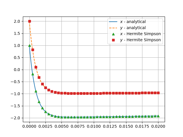
Consider the initial value problem with stiff ODE and initial condition $x(0)=1$ and $y(0)=2$ along with its analytical solution.
\[\begin{aligned} \frac{dx}{dt} &= 998x - 1998y \\ \frac{dy}{dt} &= 1000x - 2000y \end{aligned}\] \[x(t) = -2e^{-2t} + 3e^{-1000t}\] \[y(t) = -e^{-2t} + 3e^{-1000t}\]The python script below numerically solves a stiff system of linear initial value ordinary differential equations ($\dot{z} = Az$) over $t \in [0, 0.02]$ using Hermite-Simpson implicit collocation, reformulating the root-finding problem as a zero-objective nonlinear program (NLP) solved with SciPy’s Sequential Least Squares Programming (SLSQP) optimizer. The state trajectories are discretized over 40 time intervals, treating node values as decision variables and enforcing equality constraints for the initial conditions and Hermite-Simpson defect equations. Finally, it evaluates the analytical solution on a fine grid and plots both numerical trajectories ($x$ and $y$) against the exact closed-form solution to visually verify the collocation method’s accuracy.
import numpy as np
from scipy.optimize import minimize
import matplotlib.pyplot as plt

#ode equations and solution

z0 = np.array([1.0, 2.0])
A = np.array([[998, -1998],
              [1000, -2000]])
def ode(z):
    return A @ z

def analytical(t):
    x = -2 * np.exp(-2 * t) + 3 * np.exp(-1000 * t)
    y = -1 * np.exp(-2 * t) + 3 * np.exp(-1000 * t)
    return np.column_stack((x, y))

# discrete time
t_start = 0.0
t_end = 0.02
N = 40  # Number of intervals
t_nodes = np.linspace(t_start, t_end, N + 1)
h = (t_end - t_start) / N

# solving nonlinear equation == solving equality constrained optimization problem with zero objective
def objective(vars):
    return 0.0

# discrete state values at the time grid are decision variables
# vars is decision vector
# transform to appropriatte shape for collocation
# vars = [x1 y1 x2 y2...xn yn]
# Z=[[x1 y1], [x2 y2]...[xn yn]]
def constraints(vars):
    # uses row major IMP
    # every row is the state at ith time grid
    Z = vars.reshape((N + 1, 2))
    # compute derivative at all grids
    F = np.zeros_like(Z)
    for i in range(N + 1):
        F[i] = ode(Z[i])

    # assemble constraints
    cons = []
    # initial condition
    cons.extend(Z[0] - z0)
    # Hermite-Simpson collocation
    for i in range(N):
        x_i = Z[i]
        x_next = Z[i+1]
        f_i = F[i]
        f_next = F[i+1]
        x_mid = 0.5 * (x_i + x_next) + (h / 8.0) * (f_i - f_next)
        f_mid = ode(x_mid)
        #defect from collocation
        defect = x_next - x_i - (h / 6.0) * (f_i + 4.0 * f_mid + f_next)
        cons.extend(defect)
    return np.array(cons)

# from analytical solution it decays to zero from IVP
# use linear interpolation of the state as guess
initial_guess = np.zeros((N + 1, 2))
initial_guess[:, 0] = np.linspace(z0[0], 0, N + 1)
initial_guess[:, 1] = np.linspace(z0[1], 0, N + 1)
initial_guess = initial_guess.flatten()

# scipy NLP solver with some numerical settings
res = minimize(objective, initial_guess, constraints={'type': 'eq', 'fun': constraints}, method='SLSQP', options={'maxiter': 500, 'ftol': 1e-9,'disp':True})
print(res.success)
# extract the state matrix from decision vector
Z_sol = res.x.reshape((N + 1, 2))

# numerical value of analytical solution on a dense time grid
t_dense = np.linspace(t_start, t_end, 400)
Z_exact = analytical(t_dense)

plt.figure()
plt.plot(t_dense,Z_exact[:,0],'-',label=r'$x$ - analytical')
plt.plot(t_dense,Z_exact[:,1],'--',label=r'$y$ - analytical')
plt.plot(t_nodes,Z_sol[:,0]  ,'^',label=r'$x$ - Hermite Simpson')
plt.plot(t_nodes,Z_sol[:,1]  ,'s',label=r'$y$ - Hermite Simpson')
plt.legend()
plt.grid()
plt.show()
Optimization terminated successfully    (Exit mode 0)
            Current function value: 0.0
            Iterations: 2
            Function evaluations: 167
            Gradient evaluations: 2
True